26 Nov 2018
One of the most popular activation function nowadays is the REctified Linear
Unit (RELU),
defined by $f(x) = \max(0,x)$. One of the first obvious criticism is its
non-differentiability at the origin. A smooth approximation is the
softplus
function, $f(x) = log(1 + e^x)$. However, the use of softplus is discouraged by
deep learning experts. I’m wondering if a continuation scheme on the softplus
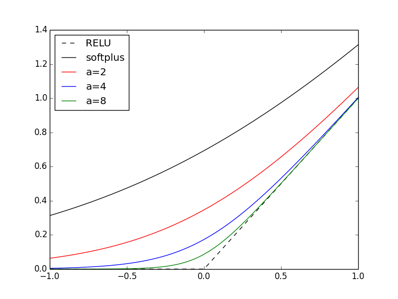
could help during training. Instead of softplus, we could use a “smooth RELU”
defined as
\[f_\alpha(x) = \frac1{\alpha} log(1 + e^{\alpha x})\]
And starting with $\alpha = 1$, i.e., the softplus function, we increase
$\alpha$ after each epoch with the effect of smoothly converging toward RELU. In
the plot below, I show RELU, softplus, and 3 examples of smooth RELUs for
$\alpha=2,4,8$.
26 Nov 2018
In this post, I want to summarize a few results about
convolution
and/or
cross-correlation.
Note that all results are derived for real functions. To work
in the complex space, one needs to take the conjugate where appropriate (e.g, in
the inner product).
Definitions
Let’s not worry about regularity and assume with only work with
$\mathcal{C}^\infty(\mathbb{R})$
functions. This out of the way, we define the
convolution of two functions $f,g$ as
\[\begin{align}
(f \star g)(t) & = \int_{- \infty}^{\infty} f(s) g(t-s) ds \\
& = \int_{- \infty}^{\infty} f(t-s) g(s) ds
\end{align}\]
The convolution operation commutes, i.e., $f \star g = g \star f$.
Next, we define the cross-correlation of two (real) functions $f,g$ as
\[\begin{align}
(f \star g)(t) & = \int_{- \infty}^{\infty} f(s) g(t+s) ds \\
& = \int_{- \infty}^{\infty} f(s-t) g(s) ds \\
\end{align}\]
Cross-correlation is the adjoint operation of convolution
Before we talk about the adjoint, we need to define (1) what operator we’re
talking about, and (2) what inner product we’re using. Given a function $f$,
let’s define the convolution operator $C_f: \mathcal{C}^\infty(\mathbb{R})
\rightarrow \mathcal{C}^\infty(\mathbb{R})$ as $C_f(g) = f \star g$.
And similarly we define the cross-correlation operator for $f$ as $D_f$.
For the inner-product on $\mathcal{C}^\infty(\mathbb{R})$, we use $\langle f, g
\rangle = \int_{-\infty}^{\infty} f(t) g(t) df$. Then for any $f,g,h$,
\[\begin{align*}
\langle C_f(g), h \rangle
& = \int_{-\infty}^{\infty} \int_{-\infty}^{\infty} f(s) g(t-s) ds \, h(t) dt \\
& = \int_{-\infty}^{\infty} \int_{-\infty}^{\infty} f(t-s) g(s) h(t) \, ds dt \\
& = \int_{-\infty}^{\infty} \int_{-\infty}^{\infty} f(t-s) h(t) dt \, g(s) ds \\
& = \int_{-\infty}^{\infty} \int_{-\infty}^{\infty} f(t) h(t+s) dt \, g(s) ds \\
& = \int_{-\infty}^{\infty} D_f(h)(s) g(s) ds \\
& = \langle g, D_f(h) \rangle
\end{align*}\]
By definition of the adjoint
of an operator, this shows that $C_f^* = D_f$.
Convolution in image processing
A classical technique for edge detection is to take finite-difference derivatives
of the discrete image.
This can also be used for edge sharpening.
In the example below, I plot the logistic function
$\sigma(x)$ (“original”)
along with the logistic function minus its second derivative, $\sigma(x) -
d^2 \sigma(x)/dx^2$ (“sharpened”).
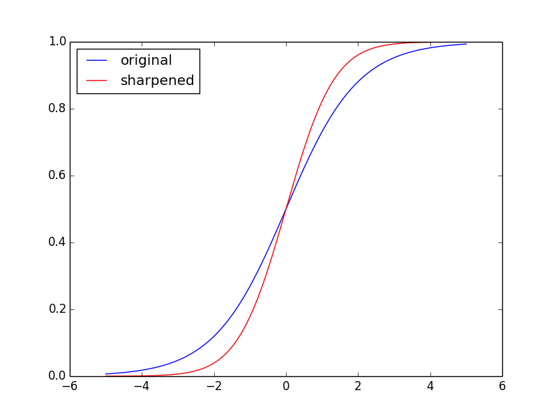
This can be formulated as taking convolution with a
specific kernel.
First of all, let’s define a discrete convolution. Typically, the scaling
factors coming from discretization are ignored, and since we’re integrating over
the whole real line there is no boundary case, therefore the discrete
convolution between functions defined over the $\mathbb{Z}$ integers, $f,g$, is
\[(f \star g)[n] = \sum_{m=-\infty}^{\infty} f[m] g[n-m]\]
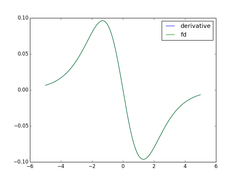
In the case of the Laplacian operator (in 1D), we can use the kernel $f$ where
all entries are zero except the ones at ${-1,0,1}$ which are equal to $[1, -2,
1]$. In the plot below, I compare the second derivative of the logistic function
with the convolution of the logistic function with the Laplacian kernel
described here. Note that I rescaled the convolution by $1/h^2$ where $h$ is the
grid size (the distance between consecutive evaluation of the function. We see
that both curvs are on top of each other. The convolution with the discrete
Laplacian could therefore
be used for edge sharpening (or edge detection) as we showed in the previous
example.
23 Nov 2018
Notations are defined in that post.
A very popular activation function for classification with a deep net is the
softmax, which is defined as
\[{\bf a}^l = [ \frac{\exp(a^{l-1}_1)}{\sum_{i=1}^{n_{l-1}} \exp(a^{l-1}_i)},
\dots,
\frac{\exp(a^{l-1}_{n_{l-1}})}{\sum_{i=1}^{n_{l-1}} \exp(a^{l-1}_i)} ]^T\]
That is ${\bf a}^l = F^l({\bf a}^{l-1})$ with
$F^l(x) = [f_1(x), \dots, f_{n_l}(x)]^T$ where
\[f_i(x) = \frac{\exp(x_i)}{\sum_j \exp(x_j)}\]
That type of activation function is different to what was covered in that
post for 2 reasons: (1) it does not have any
parameters to optimize, and (2) each coordinate depends on all other
coordinates. Let’s see how we back-propagate the gradient in that case.
For the output layer, which is the most common use-case for a softmax layer,
we need to modify the chain-rule to skip the output layer and start instead at
layer $L-1$,
\[\frac{\partial c}{\partial {\bf b}^{L-1}} =
\frac{\partial {\bf a}^{L-1}}{\partial {\bf b}^{L-1}}
\frac{\partial {\bf a}^{L}}{\partial {\bf a}^{L-1}}
\frac{\partial c}{\partial {\bf a}^{L}}\]
The only term that was not covered previously is \(\frac{\partial {\bf
a}^{L}}{\partial {\bf a}^{L-1}}\) which is simply the gradient of $F^L$.
For a hidden layer, which is definitely not the most common case for a
softmax activation function but could the case of another type of function, we
have
\[\begin{align*}
\frac{\partial c}{\partial {\bf b}^{l-1}} & =
\frac{\partial {\bf a}^{l-1}}{\partial {\bf b}^{l-1}}
\frac{\partial {\bf a}^{l}}{\partial {\bf a}^{l-1}}
\frac{\partial {\bf z}^{l+1}}{\partial {\bf a}^{l}}
\frac{\partial c}{\partial {\bf z}^{l+1}} \\
& = \frac{\partial {\bf a}^{l-1}}{\partial {\bf b}^{l-1}}
\frac{\partial {\bf a}^{l}}{\partial {\bf a}^{l-1}}
\frac{\partial {\bf z}^{l+1}}{\partial {\bf a}^{l}}
\frac{\partial c}{\partial {\bf b}^{l+1}} \\
\end{align*}\]
Again, the only term we didn’t before is \(\frac{\partial {\bf a}^{l}}{\partial
{\bf a}^{l-1}}\), which is the gradient of $F^l$.
23 Nov 2018
This post is a simple summary of some common loss functions, and their relations
to maximum likelihood estimation (MLE).
Given the data \(\{ ({\bf x}_i, {\bf y}_i) \}_i\),
and model parameters $\theta$,
we define a general loss function as
\[\mathcal{L}(\{ \theta \}) =
\frac1N \sum_{i=1}^N
c(\theta; {\bf x}_i, {\bf y}_i)\]
We also assume that that model make the predictions
\({\bf f}(\theta; {\bf x}_i)\).
Regression
In a regression setting, a very common choice is a least-square loss function,
or $L_2$ loss function,
i.e.,
\[c(\theta; {\bf x}_i, {\bf y}_i)
= \frac12 \| {\bf f}(\theta; {\bf x}_i) - {\bf y}_i \|^2\]
To calculate the gradient of the loss function, we need the partial derivative
of $c$ with respect to the output of the model $f$, which in this case is
\[\frac{\partial c(\theta; {\bf x}_i, {\bf y}_i)}{\partial {\bf f}(\theta; {\bf
x}_i)} = {\bf f}(\theta; {\bf x}_i) - {\bf y}_i\]
The main advantage of that loss function is its simplicity. Linear regression
with that loss function can be solved analytically. The least-square loss
function is twice differentiable everywhere. In the case of a model with
Gaussian noise, it also connects with MLE. Indeed, if we assume that the true
model is
\[{\bf y}_i = {\bf f}(\theta; {\bf x}_i) + \varepsilon\]
with $\varepsilon$ having a normal distribution with mean zero, then minus the
log-likelihood is given by
\[\frac{n}2 \log(2 \pi \sigma^2) + \frac1{2\sigma^2} \sum_i
\| {\bf f}(\theta; {\bf x}_i) - {\bf y}_i \|^2\]
A disadvantage of the least-square loss function is its sensitivity to outliers.
Indeed, if the \(k^\text{th}\) data point is an outlier, the square deviation
will dominate the loss function and during the training phase, the optimization
will give too much importance to that data point in an attempt to minimize the
loss function. This is related to the fact that the least-square targets the
mean of the distribution, which is sensitive to outliers.
This is in contrast to the $L_1$ loss function, which targets the median the
distribution, and is
\[c(\theta; {\bf x}_i, {\bf y}_i)
= | {\bf f}(\theta; {\bf x}_i) - {\bf y}_i |\]
The main disadvantage of the $L_1$ loss function is its numerical difficulties.
It is non-differentiable at the origin, and requires specific techniques to be
handled.
Binary classifier
Typically, loss functions for binary classification derive from MLE. Assuming the
binary classes are \(y_i \in \{0,1\}\), and assuming that the classifier
returns a function \(f({\bf x}_i) \in [0,1]\) which can be interpreted as
\(\mathcal{P}[f({\bf x}_i) = 1 | \theta]\), then the likelihood function is
given by
\[\begin{align*}
& \prod_i (f({\bf x}_i))^{\mathcal{1}_{\{y_i=1\}}}
(1-f({\bf x}_i))^{\mathcal{1}_{\{y_i=0\}}} \\
= & \prod_i (f({\bf x}_i))^{y_i} (1-f({\bf x}_i))^{1-y_i}
\end{align*}\]
So either $y_i=1$ and we have only the first term, or $y_i=0$ and we have the
second term.
This is the general way of writing the likelihood function for a Bernoulli
distribution which returns value $1$ with probability $f({\bf x}_i)$ and value
$0$ with probability $1-f({\bf x}_i)$.
Then the negative log-likelihood is
\[- \sum_i y_i \log(f({\bf x}_i)) + (1-y_i) \log(1-f({\bf x}_i))\]
Let’s look at an example. In the case of a logistic regression, the model is
given by
\[f({\bf x}_i) = \frac1{1 + e^{-{\bf x}_i^T \theta}}\]
In that case, the negative log-likelihood is
\[\begin{align*}
& = y_i \log (1 + e^{-{\bf x}_i^T \theta})
-(1-y_i) (-{\bf x}_i^T \theta - \log(1 + e^{-{\bf x}_i^T \theta}) \\
& = - y_i {\bf x}_i^T \theta + \log(1 + e^{+{\bf x}_i^T \theta})
\end{align*}\]
In the case we have multiple classes \(y_i \in \{0,1,\dots,K-1\}\) and multiple
outputs \({\bf f}({\bf x}_i) \in [0,1]^K\),
and all outputs are mutually exclusive (i.e., they always sum to $1$, as is the
case when using softmax in a neural network),
we have the interpretation that
\({\bf f}({\bf x}_i)_j = \mathcal{P}({\bf f}({\bf x}_i) = y_j | \theta)\).
The loss function is typically defined as
\[c(\theta; {\bf x}_i, y_i) = - \sum_{j=0}^K \mathcal{1}_{\{y_i = j\}} \log (
\mathcal{P}({\bf f}({\bf x}_i) = j | \theta) )\]
\[c(\theta; {\bf x}_i, y_i) = - \log( {\bf f}({\bf x}_i)_{y_i} )\]
In that case, the partial derivative of the $c$ with respect to the output of
the model is
\[\frac{\partial c(\theta; {\bf x}_i, y_i)}{\partial {\bf f}(\theta; {\bf x}_i)} =
[\dots,0,- 1/{\bf f}({\bf x}_i)_{y_i},0,\dots]^T\]
It is interesting to note that these loss functions are often called
cross-entropy, as they can be derived from information theory.
13 Nov 2018
As a learning tool, and inspired by that interesting
article, I want to build my own artificial
neural network in Python.
Notations
The first step is define all the notations I’m going to use.
Layers are indexed by $l=0,1,\dots,L$.
The input layer is indexed by $0$, and the output layer is $L$. In each layer $l$,
we have $n_l$ neurons, each producing an output $a^l_i$ for $i=1,\dots,n_l$.
All outputs from layer $l$ are stored in the vector ${\bf a}^l =
[a^l_1,\dots,a^l_{n_l}]^T$.
In layer $l$, each neuron takes an affine combination of the $n_{l-1}$ outputs
from the previous layer, then pass them through an activation function
$f: \mathbb{R} \rightarrow \mathbb{R}$
to produce the $n_l$ outputs. The weights of the linear
combination are denoted ${\bf w}^l_i= [w^l_{i1}, \dots, w^l_{in_{l-1}}]^T$
and the constant is denoted $b^l_i$, such
that
\[a^l_i = f(({\bf w}^l_i)^T {\bf a}^{l-1} + b^l_i )\]
Let’s shorten the notations a bit using vectorial notations. Let’s define the total
activation function for layer $l$ as $F^l: \mathbb{R}^{n_l} \rightarrow
\mathbb{R}^{n_l}$ with $F^l(x) = [f(x_1), \dots, f(x_{n_l})]^T$. Let’s
introduce the weight matrix at layer $l$, ${\bf W}^l = [{\bf w}^l_1, \dots, {\bf
w}^l_{n_l}]^T \in \mathbb{R}^{n_l \times n_{l-1}}$,
and the constant vector ${\bf b}^l = [b^l_1, \dots, b^l_{n_l}]^T$.
We can then write, for $l=1,\dots,L$,
\[{\bf a}^l = F^l \left({\bf W}^l \cdotp {\bf a}^{l-1} + {\bf b}^l \right)\]
I’ll introduce one last variable to simplify the notation. Let’s call ${\bf
z}^l$ the input for layer $l$, i.e.,
\[{\bf z}^l = {\bf W}^l \cdotp {\bf a}^{l-1} + {\bf b}^l\]
Then we can write the activation at layer $l$ as,
\({\bf a}^l = F^l \left( {\bf z}^l \right)\).
The only exception is for the input layer $l=0$ where $a^0$ is not calculated
but is an input variable.
At every layer, we therefore have $n_l (n_{l-1} + 1)$ parameters for a
grand total of $\sum_{l=1}^N n_l ( n_{l-1}+1)$ parameters in the entire network.
Loss function
To train the network, we need to define a loss function. Let’s assume we have
data \(\{ ({\bf x}_i,{\bf y}_i) \}_{i=1}^N\), where ${\bf x}_i$ is fed in the input
layer and ${\bf y}_i$ is compared with the output of the network. The output of
the network is therefore a function of all parameters and the input variable,
i.e., \({\bf a}^L = {\bf a}^L( \{ {\bf W}^l, {\bf b}^l \}_l; {\bf x})\).
For the loss function, I will use a least-square misfit, which leads to
\[\mathcal{L}(\{ {\bf W}^l, {\bf b}^l \}_l) =
\frac1{2N} \sum_{i=1}^N
\| {\bf a}^L( \{ {\bf W}^l, {\bf b}^l \}_l; {\bf x}_i) - {\bf y}_i \|^2\]
To estimate the loss function, we simply plug, for each data pair $({\bf x}_i,
{\bf y}_i)$, the input ${\bf x}_i$ in the input layer, i.e., we set ${\bf a}^0 =
{\bf x}_i$, then propagate that forward sequentially. To emphasize the
dependence on a specific data point, we write ${\bf a}^k = {\bf a}^k({\bf
x}_i)$,
\[\begin{align*}
{\bf a}^1({\bf x}_i) & = F^1({\bf W}^1 {\bf x}_i + {\bf b}^1) \\
{\bf a}^2({\bf x}_i) & = F^2({\bf W}^2 {\bf a}^1({\bf x}_i + {\bf b}^2) \\
\vdots & \\
{\bf a}^L({\bf x}_i) & = F^L({\bf W}^L {\bf a}^{L-1}({\bf x}_i) + {\bf b}^L)
\end{align*}\]
Similarly we denote \({\bf z}^k = {\bf z}^k({\bf x}_i) =
{\bf W}^k {\bf a}^{k-1}({\bf x}_i) + {\bf b}^k\).
And we decompose the loss function into
\(\mathcal{L}(\{ {\bf W}^l, {\bf b}^l \}_l) =
1/N \sum_{i=1}^N c(\{ {\bf W}^l, {\bf b}^l \}_l, {\bf x}_i)\) where
\[c(\{ {\bf W}^l, {\bf b}^l \}_l, {\bf x}_i) =
\frac12 \| {\bf a}^L( \{ {\bf W}^l, {\bf b}^l \}_l; {\bf x_i}) - {\bf y}_i \|^2\]
Calculating derivatives
To minimize the loss function, we need to calculate derivatives of that loss
function $L$ with respect to the parameters ${\bf W}^l$ and ${\bf b}^l$ at each
layers. This is done via the backpropagation algorithm; for more details on the
backpropagation, see this post.
The main results are that, after a forward propagation (see previous section),
the gradient of the loss function can be calculated as
\[\begin{align*}
\frac{\partial \mathcal{L}}{\partial {\bf b}^l} & = \frac1N \sum_{i=1}^N
\frac{\partial c({\bf x}_i)}{\partial {\bf b}^l} \\
\frac{\partial \mathcal{L}}{\partial {\bf W}^l} & = \frac1N \sum_{i=1}^N
\frac{\partial c({\bf x}_i)}{\partial {\bf W}^l}
\end{align*}\]
For each contribution $c({\bf x}_i)$ to the loss function, its derivatives
with respect to all parameters can be
calculated sequentially starting from the output layer $L$, and moving backward
to the first layer, by using the formulas for each $i=1,\dots,N$,
\[\begin{align*}
\frac{\partial c({\bf x}_i)}{\partial {\bf b}^L} & =
\begin{bmatrix} f'( z_1^L({\bf x}_i) ) & & 0 \\ & \ddots & \\ 0 & & f'(z_{n_L}^L({\bf x}_i))
\end{bmatrix} \cdotp
\frac{\partial c({\bf x}_i)}{\partial {\bf a}^L}
\\
\frac{\partial c({\bf x}_i)}{\partial {\bf b}^l} & = \begin{bmatrix}
f'( z_1^l({\bf x}_i) ) & & 0 \\ & \ddots & \\ 0 & & f'(z_{n_l}^l({\bf x}_i))
\end{bmatrix} \cdotp ({\bf W}^{l+1})^T \cdotp \frac{\partial c({\bf x}_i)}{\partial {\bf
b}^{l+1}} , \quad \forall l=1,\dots,L-1\\
\frac{\partial c({\bf x}_i)}{\partial {\bf W}^l} & =
\frac{\partial c({\bf x}_i)}{\partial {\bf b}^l} \cdotp ({\bf a}^{l-1}({\bf x}_i))^T ,
\quad \forall l=1,\dots,L
\end{align*}\]
Initialization
Initialization is quite critical to the success of neural nets.
Typically, all biases ${\bf b}^l$ are initialized to zero.
You however don’t want to do that with the weights, or you’d effectively kill
all layers (see post). Also, you want to make sure that
you do not saturate all neurons, for all data points. For that reason, you tend
to choose random values centered around zero. And this must go along with
normalized input data, to avoid immediate saturation of neurons. There are a few
heuristic to choose an weight initialization distribution.
Symmetry
If in a layer one uses the exact same weights for each neuron (either at
initialization, or during the optimization), then all neurons of that layer
will remain the same. That is apparent when looking at the derivatives. Whatever
the vector misfit (for the output layer), or the derivative from the layer just
after, if all weights are the same, the derivative will be the same. It is
therefore important to “break the symmetry” in the initialization.
Implementation
I implemented all those ideas from scratch in Python;
The code is available on GitHub.
You can use it to assemble a neural network and calculate its derivatives using
the backpropagation algorithm.