Notes for CNN course by deeplearning.ai (week 2)
23 Jan 2021These are my notes for week 2, focusing on case studies.
Video: Why look at case studies?
Look at classic CNN is a good way to gain intuition about how CNNs work. Also, in computer vision, successful architecture for one task is often good for another task.
Classic CNN examples looked at this week:
- LeNet-5
- AlexNet
- VGG
- ResNet
- Inception
Video: Classic Networks
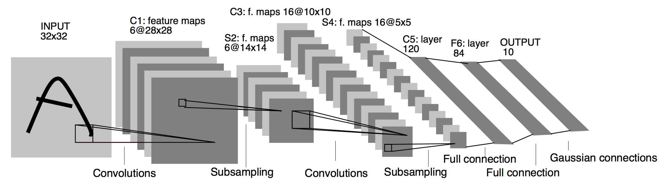
LeNet-5 (1998)
Introduced to recognize black&white hand-written digits (32x32x1). The architecture is described below. Note that at the time of the paper, padding was not common. So all convolutional layers shrink the size of the image.
- Convolutional layer: 5x5, stride=1, 6 channels -> output: 28x28xg
- average pooling (today would probably use max pooling): 2x2, stride=2 -> output: 14x14x6.
- Convolutional layer: 5x5, stride=1, 16 channels -> output: 10x10x16
- average pooling : 2x2, stride=2 -> output: 5x5x16.
- fully connected layers: 400x120, 120x84, 84x10.
- output layer today would probably be a softmax. In the paper, they used something else that is not common today.
All non-linearities were tanh or sigmoid. Also, they applied activation functions after the pooling layers. Total network had about 60,000 parameters, which is small by today’s standard (>1M parameters). However variation in image size through the network remains current: height and width go down, number of channels go up. Another aspect that remains often true today is the alternance of the layers: conv, pool, conv, pool, fc, output. A last note, they had a different way of apply the kernels to the input image (i.e, didn’t have kernels with the same number of channels as the input).
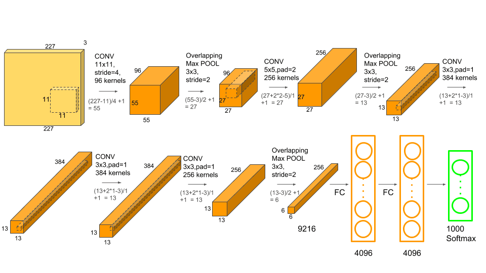
AlexNet (2012)
The architecture is described below. The input image is 227x227x3.
- conv layer, 11x11, stride=4, 96 channels -> 55x55x96
- max pooling, 3x3, stride=2 -> 27x27x96
- conv layer, 5x5, same padding, 256 channels -> 27x27x256
- max pooling, 3x3, stride=2 -> 13x13x256
- conv layer, 3x3, same padding, 384 channels ->13x13x384
- conv layer, 3x3, same padding, 384 channels ->13x13x384
- conv layer, 3x3, same padding, 256 channels ->13x13x256
- max pooling, 3x3, stride=2 -> 6x6x256
- conv layer, 3x3, same padding, 384 channels ->13x13x384
- conv layer, 3x3, same padding, 384 channels ->13x13x384
- conv layer, 3x3, same padding, 256 channels ->13x13x256
- Fully-connected layers: 9216 -> 4096 -> 4096 -> 1,000 (Softmax)
Many similarities with LeNet-5, but AlexNet has about 60M parameters. Also, they used ReLU activation functions. They also used another type of layer called Local Response Normalization, which normalizes each pixel/position across all channels. This type of layer is not really used anymore as it was found that it had a very small impact on the results.
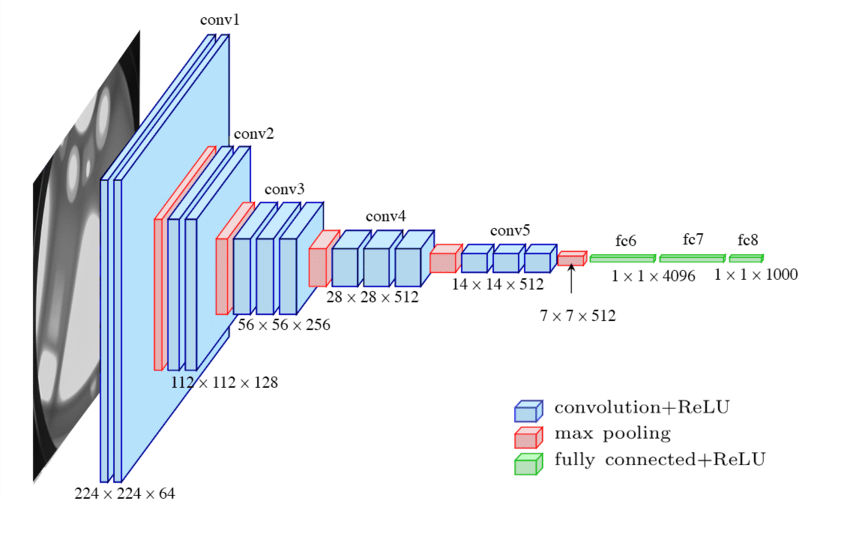
VGG-16 (2015)
The architecture can be visualized here. VGG-16 really simplified the neural networks architecture. It only relies on a single type of convolutional layer (3x3, stride=1, same padding) and a single type of max pooling (2x2, stride=2). The input is 224x224x3.
- conv: 64 channels
- conv: 64 channels -> 224x224x64
- max pooling -> 112x112x64
- conv: 128 channels
- conv: 128 channels -> 112x112x128
- max pooling -> 56x56x128
- conv: 256 channels
- conv: 256 channels
- conv: 256 channels -> 56x56x256
- max pooling -> 28x28x256
- conv: 512 channels
- conv: 512 channels
- conv: 512 channels -> 28x28x512
- max pooling -> 14x14x512
- conv: 512 channels
- conv: 512 channels
- conv: 512 channels -> 14x14x512
- max pooling -> 7x7x512
- fc: 4096 -> 4096 -> 10,000 (softmax)
VGG-16 has about 138M parameters, which is large even by today’s standards. 16 is the number of layers. There is also a VGG-19, but performance is comparable. VGG is attractive to the community b/c it simplifies the construction of the network by systematizing the change in height/width and channels from one layer to the next.
Video: ResNets (2016)
ResNets was introduced to help training of very deep neural networks. In practice, we notice that training error for plain network will start to increase after a certain depth is reached. ResNets allows to train networks of 100 or 1,000 layers deep and still see the training error gradually decrease as the depth of the network increases. ResNets helps with the problems of vanishing and exploding gradients.
Elementary block of a ResNet is a Residual Block, which adds a skip connection (or shortcut) to typical fully-connected layers. In a given layer, after the linear part but before the application of the ReLU activation function, the value of layer output a few levels below is added, eg, $a^{[l+2]} = g(z^{[l+1]} + a^{[l]})$.
Video: Why ResNets work?
Uses an intuitive example to try and show why ResNets work. Intuition is that ResNets can very easily learn the identity map (W=0, b=0). That means, it’s easy for a ResNets layer plugged after an existing DL to do at least as well. Then after training, it’s easy to imagine that the addition of the ResNets will improve performance.
Something else to notice about ResNets is that you need to have $z^{[l+2]}$ and $a^{[l]}$ that have same dimension. For that reason, you often see people using the same convolution (or same padding). However, this is not mandatory, as one can add a linear transformation of $a^{[l]}$ so that its dimension match with $z^{[l+2]}$. That linear transformation can be learned or fixed (eg, padding,…).
Video: Networks in Networks and 1x1 Convolutions
In the paper Network in Network, they discuss the use of a 1x1 convolution. It’s interesting in the case of a multi-channel image, where it takes a linear combination of each channels (before passing it through a non-linear activation function).
This idea of 1x1 convolution can be used to shrink the number of channels of an image w/o altering the height or width. altering
Video: Inception Network Motivation
Main motivation is that instead of choosing amongh a 1x1 convolution, a 3x3 convolution, a 5x5 convolution, or a max-pooling layer, why don’t you just do them all in a single layer. Then stack all the outputs along the channel dimension. That’s what the inception layer is about. You of course need same padding to preserve the height and width and be able to stack them along the channel dimension.
Problem of that approach is the computational cost. For instance, 5x5 conv with same padding, going from 28x28x192 to 28x28x32 involves about 120M fp operations. A solution is to introduce a bottleneck layer, that is 1x1 convolution that reduces the number of channles (eg, from 192 down to 16). Then apply the 5x5 convolution on that output with a reduced number of channels. You can reduce the computational cost by 1/10th.
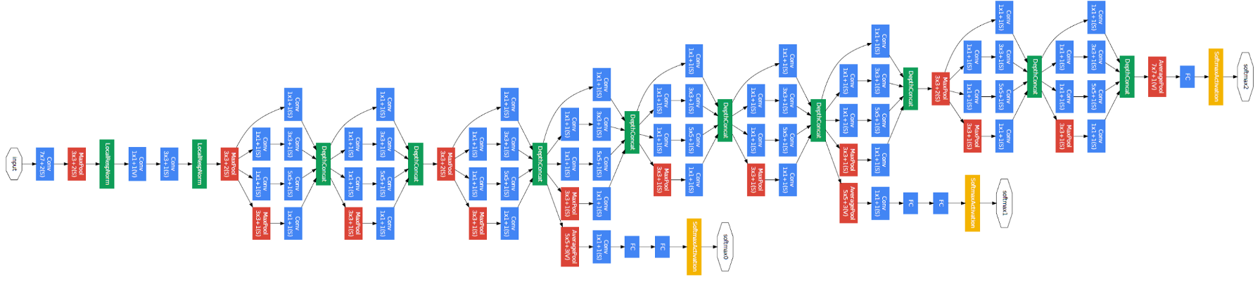
Video: Inception network
A visualization of the architecture of the inception network can be found here.
Rough idea is as descrbied in the previous section: apply 1x1, 3x3, 5x5 convolutions, and max-pooling in parallel, the concatenate all the channels together. To reduce computational cost, 3x3 and 5x5 convolutional layers are preceded by a bottleneck layer, and to avoid having max-pooling dominate the output, it is followed by a bottleneck layer. All of this represents an inception module. The inception network is more or less a stack of multiple inception modules.
A noticeable addition is that you find intermediate probes in the network that try to predict the outcome with a sequence of fully-connected layers followed by a softmax. The rationale behind that is to try and force the network to regularize itself by trying to do these intermediate predictions.
Important note: Inception was the architecture used to introduce batch norm. A few other modifications were made to the network though (learning rate, no dropout,…).
Video: Using open-source implementation
github
Video: Transfer Learning
At least in computer vision, transfer learning should always be considered unless you have an exceptionally large dataset. Transfer learning ranges from: i. keeping all layers frozen and replacing/training the output layer (eg, softmax layer) ii. keeping a few layers frozen (if you have more data) iii. re-training the entire network, starting from the trained model as initialization.
Video: Data augmentation
In most computer vision applications today, you never have enough data. Data augmentation can help “get” more data.
A few common methods:
- mirroring
- random cropping
- rotation (less common)
- shearing (less common)
- local warping (less common)
Another type of data augmentation is color shifting, where you add random perturbations to the RGB channels. Also, there is a “PCA color augmentation” (see AlexNet paper).
In terms of computational efficiency, data augmentation can be done a separate CPU thread, before passing the augmented data to the CPU/GPU used for training, which is completely paralelizable.
Note that data augmentation most often comes with a set of hyparameters that also need to be selected.
Video: State of Computer Vision
Less data means you’ll need more hand-engineering to get good results.
Other tips:
- Ensemble: good for competition or benchmark, but rarely used in production due to the computational cost
- multi-crop at test time: compute prediction for multiple cropped version of your input image, then average the results. Same problem as ensemble for production solution
cnn course deeplearning