Convolution, cross-correlation

26 Nov 2018

In this post, I want to summarize a few results about convolution and/or cross-correlation. Note that all results are derived for real functions. To work in the complex space, one needs to take the conjugate where appropriate (e.g, in the inner product).

Definitions

Let’s not worry about regularity and assume with only work with $\mathcal{C}^\infty(\mathbb{R})$ functions. This out of the way, we define the convolution of two functions $f,g$ as

\[\begin{align} (f \star g)(t) & = \int_{- \infty}^{\infty} f(s) g(t-s) ds \\ & = \int_{- \infty}^{\infty} f(t-s) g(s) ds \end{align}\]

The convolution operation commutes, i.e., $f \star g = g \star f$. Next, we define the cross-correlation of two (real) functions $f,g$ as

\[\begin{align} (f \star g)(t) & = \int_{- \infty}^{\infty} f(s) g(t+s) ds \\ & = \int_{- \infty}^{\infty} f(s-t) g(s) ds \\ \end{align}\]

Cross-correlation is the adjoint operation of convolution

Before we talk about the adjoint, we need to define (1) what operator we’re talking about, and (2) what inner product we’re using. Given a function $f$, let’s define the convolution operator $C_f: \mathcal{C}^\infty(\mathbb{R}) \rightarrow \mathcal{C}^\infty(\mathbb{R})$ as $C_f(g) = f \star g$. And similarly we define the cross-correlation operator for $f$ as $D_f$. For the inner-product on $\mathcal{C}^\infty(\mathbb{R})$, we use $\langle f, g \rangle = \int_{-\infty}^{\infty} f(t) g(t) df$. Then for any $f,g,h$,

\[\begin{align*} \langle C_f(g), h \rangle & = \int_{-\infty}^{\infty} \int_{-\infty}^{\infty} f(s) g(t-s) ds \, h(t) dt \\ & = \int_{-\infty}^{\infty} \int_{-\infty}^{\infty} f(t-s) g(s) h(t) \, ds dt \\ & = \int_{-\infty}^{\infty} \int_{-\infty}^{\infty} f(t-s) h(t) dt \, g(s) ds \\ & = \int_{-\infty}^{\infty} \int_{-\infty}^{\infty} f(t) h(t+s) dt \, g(s) ds \\ & = \int_{-\infty}^{\infty} D_f(h)(s) g(s) ds \\ & = \langle g, D_f(h) \rangle \end{align*}\]

By definition of the adjoint of an operator, this shows that $C_f^* = D_f$.

Convolution in image processing

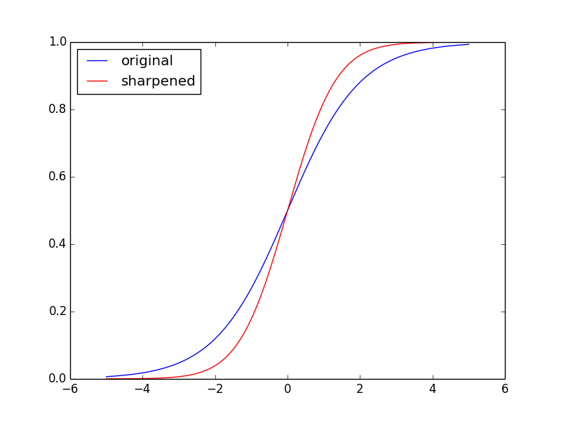
A classical technique for edge detection is to take finite-difference derivatives of the discrete image. This can also be used for edge sharpening. In the example below, I plot the logistic function $\sigma(x)$ (“original”) along with the logistic function minus its second derivative, $\sigma(x) - d^2 \sigma(x)/dx^2$ (“sharpened”).

This can be formulated as taking convolution with a specific kernel. First of all, let’s define a discrete convolution. Typically, the scaling factors coming from discretization are ignored, and since we’re integrating over the whole real line there is no boundary case, therefore the discrete convolution between functions defined over the $\mathbb{Z}$ integers, $f,g$, is

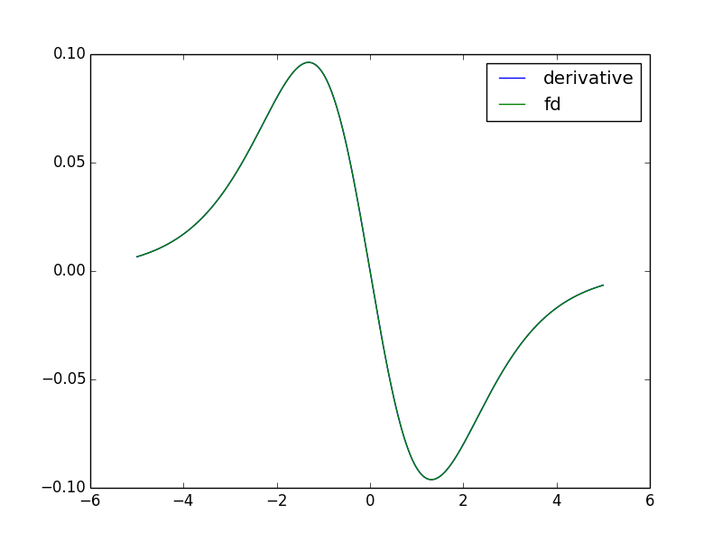
\[(f \star g)[n] = \sum_{m=-\infty}^{\infty} f[m] g[n-m]\]

In the case of the Laplacian operator (in 1D), we can use the kernel $f$ where all entries are zero except the ones at ${-1,0,1}$ which are equal to $[1, -2, 1]$. In the plot below, I compare the second derivative of the logistic function with the convolution of the logistic function with the Laplacian kernel described here. Note that I rescaled the convolution by $1/h^2$ where $h$ is the grid size (the distance between consecutive evaluation of the function. We see that both curvs are on top of each other. The convolution with the discrete Laplacian could therefore be used for edge sharpening (or edge detection) as we showed in the previous example.

[ convolution  correlation  image  ]